Research
This page summarizes my ongoing postdoctoral research supervised by Donald Estep, Director of the Canadian Statistical Sciences Institute, as well as past work during my PhD with my advisor Matey Neykov. A full list of the resulting publications can be found on my Publications page.
Stochastic Inverse Problems
At SFU, I’m studying properties of a non-parametric Bayesian approach to calibrating computer models. Suppose we observe \(q_1,\cdots,q_K\) where \(q_i=Q(\lambda_i)\) for \(\lambda_1,\cdots,\lambda_K\sim P_{\Lambda}^t\). The \(\lambda_i\) represent physical parameters that govern the behavior of a physical system modeled with \(Q\). For example, \(\lambda_i\) could be the properties of a medium through which particles travel, yielding \(q_i\) observations (particle counts), or it could be material properties of a metal being heated to give temperature observations. The goal is to produce a distribution \(\hat P_{\Lambda}\) that is consistent with the distribution of the \(q_i\) (the pushforward measure of \(P_{\Lambda}^t\)). Recent work by my advisor’s lab (Shi et al. 2025) developed an approach based on measure theory and Bayesian ideas. This method and older variants have already seen several real-world applications to difficult scientific problems, including ground-water contamination and storm surge modelling. My work thus far has been showing that the solution operator proposed is continuous in the distribution \(P_{\Lambda}^t\) as well as studying deeper implications of continuity to the theory of Bayesian statistics. I’m excited to contribute to this novel area of research, which brings together fundamental probability theory, engineering applications, and computational techniques from Bayesian statistics.
Featured Work
- Prasadan, A., Estep, D., & Bingham, D. (2026). Continuity of the Solution of a Non-Parametric Bayesian Statistical Calibration Procedure. arXiv preprint arXiv:2603.20665.
Shape-Constrained Mean Estimation
This topic was the subject of my thesis and combined several themes all at once: mean estimation, minimax optimality, shape-constraints, adversarial contamination, sub-Gaussian noise, and function classes. Let me give a brief overview.
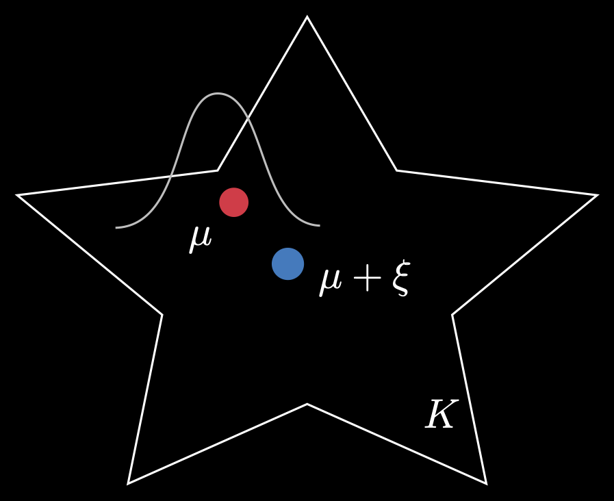
A fundamental problem in statistics is estimating some unknown signal \(\mu\) (could be a real number, vector, or function). We are given several noisy observations of the form \(Y_i=\mu+\xi_i\) where \(\xi_i\) is IID Gaussian noise. At this point, you might propose something like the average \(\overline{Y}_i\) as our estimate of \(\mu\).
Next, suppose we are told that \(\mu\) must belong to a known set \(K\). Has the problem become easier? No! Now, we must devise an algorithm that always returns an estimate in this set. This is called shape-constrained estimation.
Moreover, we want an estimate that is minimax optimal. This is a very conservative but important benchmark for assessing the performance of an estimator. In this context, we want to produce an estimator whose average performance in the worst-case choice of \(\mu\) is minimized. I said ‘average’ because there is randomness in the data generating process for \(\vec{Y}\), and worst case because \(\mu\) could, in principle, come from anywhere in \(K\). In the simple Euclidean vector case, this might be of the form: \[\inf_{\hat{\mu}} \sup_{\mu \in K} \mathbb{E}\|\hat{\mu}(\vec{Y}) - \mu\|_2^2,\] where \(\hat\mu\) ranges over the set of all estimators evaluated on my random data \(\vec{Y}\).
In this work, we devised minimax optimal techniques to estimate means when the underlying set was star-shaped (see below), a generalization of convexity. We extended this work to a non-parametric regression setting, i.e., observing \(Y_i=f^{\ast}(X_i)+\xi_i\) and trying to find \(f^{\ast}\). We also allowed for adversarial contamination of some fraction \(\epsilon<1/2\) of the data. In each of these problems, we generalized our assumptions on \(\xi_i\) to permit sub-Gaussian noise, which is a rich class of probability distributions whose tails are ‘lighter’ than Gaussians.
This thesis was ultimately one of many sequels to my advisor’s paper (Neykov 2023) which studied a convex-constrained mean estimation problem. The framework continues to inspire work, including applications in heavy-tailed noise and density estimation with contamination.
Featured Work
- Peng, T., Prasadan, A., & Neykov, M. (2026). Robust mean estimation under star-shaped constraints with heavy-tailed noise. arXiv preprint arXiv:2604.05063.
- Prasadan, A., & Neykov, M. (2026). Information theoretic limits of robust sub-Gaussian mean estimation under star-shaped constraints. The Annals of Statistics, 54(1):490 – 515.
- Prasadan, A., & Neykov, M. (2025). Some facts about the optimality of the lse in the gaussian sequence model with convex constraint. IEEE Transactions on Information Theory, 71(11):8928–8958.
- Prasadan, A., & Neykov, M. (2025). Characterizing the minimax rate of nonparametric regression under bounded star-shaped constraints. Electronic Journal of Statistics, 19(2), 3449-3488.
Multistate and Joint Models
During my PhD, I joined a collaboration between CMU and Novartis to study the use of flexible survival analysis techniques to model the efficacy of immunotherapy for blood cancers. The treatment itself sounds straight out of a sci-fi novel: scientists bioengineer immune cells to modify their own outer cell structure so the cells learn to attack cancer cells.
Classic survival analysis can be used to model the literal survival of a subject: the subject is either alive or dead, for example. But what if we wish to capture the dynamic trajectory of patients through different stages of sickness? For example, the patient might first see their condition worsening, then improving, then becoming fully cancer-free or reverting to total treatment failure. A multi-state model allows us to model a patient’s transitions between different states (of cancer), and thus is a powerful tool for evaluating cancer treatments.
The second theme of this work was joint models, which are a lot more exciting than their generic name suggests. The idea is to jointly model longitudinal and survival processes, when the longitudinal data is endogenous, or internal to the patient. Classic Cox proportional hazard models can handle time varying covariates, but they require exogeneity. This means, for example, that if the patient is censored (e.g., leaves the study or dies), then the existence of the longitudinal covariate should be unaffected. This is true if, for example, your longitudinal variable is the weather. But clearly it fails with biomarkers in your blood. With a joint model, we compute a posterior distribution over the longitudinal and survival processes that gives theoretically valid estimates unlike the regular Cox proportional hazard model.
I used this work to satisfy our PhD program’s requirement of completing an “Advanced Data Analysis” project. I worked with Joel Greenhouse at CMU as well as a team of statisticians at Novartis for about 2 years. I also presented some of our work on joint models at the 2023 Joint Statistical Meetings in Toronto.
Featured Work
- Prasadan, A., James, D. A., & Greenhouse, J. (2022) “Assessing CAR-T immunotherapy outcomes using multistate models, pharmacokinetics, and tumor burden.” Novartis Technical Report.
- Invited Topics Contributed Session, Joint Statistical Meetings (JSM), Toronto, 2023. “Joint modeling of transduced cellular kinetics, tumor size, and survival endpoints.”